What skills do you need for data science?

Data science is one of the best jobs out there. You work with fascinating datasets on practical, intellectually stimulating problems. It's no wonder that for US News & World Report give it consistently high marks, the US Bureau of Labor Statistics predict excellent job growth over the next decade (15%, above the national average of 4%), and, for the last five years, data science has ranked in the top three of 50 Best Jobs in America by glassdoor.

So, what does it take to be a data scientist? In the inaugural post of this blog, I thought we'd look into the skills employers are seeking.

1. Question

What are the most commonly sought-after skills for data scientists?

2. Approach

While there are many informative posts on data science blogs about necessary skills for an aspiring data scientist, here we will have a more quantitative look at in-demand skills. We are going to look directly at job postings.

Since there is no online dataset of data science job postings that I'm aware of, we'll need to perform a simple web scraping exercise to gather the data ourselves. We'll collect data from Indeed, which supposedly has listings for >25k jobs in data science at the time of this writing. Given that there were only ~33k total data science jobs in the US in 2019, this number seems a bit fishy. So, the next part of our job will be to clean up the dataset.

3. Data collection

We will gather information on data science job postings using a simple web scraping python script using the beautifulsoup library.

First, we want to explore the website and perform a few searches. This will enable us to learn the url structure, which we need to understand in order to loop through search results.

Fortunately, the job searches have a simple to understand structure (below).
https://www.indeed.com/jobs?q=data+science&start=

By default, 10 job pages are shown. So if we want to step through search results, we would put 0 at the end of the above url, then 10, 20, 30, etc. This works, but it would be better to display more results in order to load fewer pages. In the "Advanced Job Search" page, there is an option to increase results displayed per page to 50. It modifies the url in a simple way.
https://www.indeed.com/jobs?q=data+science&limit=50&start=

This will be our base url that we will loop through when performing our scrape. It is important to note that the order of job results is not reproduceable. Jobs are commonly being added, and the order results are displayed is controlled by Indeed. What this means for us is that our search may miss some job postings, and it may pull the same posting more than once. Neither is much of a problem for our analysis. We want a large number of postings, but we do not need all of the postings. So, we just will want to run this script a few times over the course of two or three days. We'll end up with a lot of duplicates, which can easily remove later.

Now, we're ready to code the scraper. I'll walk through some of the code below. You can find the code in its entirety, and the results of the job scrape, on GitHub.

We'll be using python 3. First, we need to import the following libraries.

from urllib.request import Request, urlopen
from bs4 import BeautifulSoup
import pandas as pd
import time
from datetime import datetime, timedelta

Next, we define some of our variables. You'll note that we are storing our scraped data in a variable named data, which includes data we scrape on the job title, date posted, company name, star rating of the company, location, salary, description, and posting link. This is more information than we need to answer our question, but since we are here already, might as well scrape all of the tangential data. The other information could come in handy down the line.

# This is where we record our data
data = [ [] for i in range(8) ] # 0:Title, 1: Date posted, 2:Company, 3:Rating, 4:Location, 5:Salary, 6:description, 7:Link

# Record the time the search initiated and put the output time in the file name
now = datetime.now()
now_str = now.strftime("%Y-%m-%d_%H-%M-%S")
out = ''.join(['jobs_', now_str, '.ftr'])

#This is the base url for searches
search_base = 'https://www.indeed.com/jobs?q=data+science&limit=50&start='

We then loop through the results pages. In each loop, we will modify the base url by concatenating the number of jobs we have scraped. We then load the webpage and create a soup object.

# Perform search and create a soup object
search_url = ''.join([search_base,str( len(data[0]) )])
html = Request(search_url, headers={'User-Agent': 'Mozilla/5.0'})
time.sleep(3) # Allow 3 seconds for the search to occur
page = urlopen(html)
content = page.read()
soup = BeautifulSoup(content, 'html.parser')

We'll refer to each job posting displayed on the a search results page as a job card. We want to find all of the job cards on each search result page. The way that we find the relevant html code for identifying the job cards is to perform the search in our normal browser (e.g., chrome, edge, etc.), right click the page, and select view source or, even better, inspect.

# Locate job cards
flag = 0 # 0: No popup, 1: Popup
cards = soup.findAll('div', attrs={'class': 'jobsearch-SerpJobCard unifiedRow row result'})
if len(cards) == 0: # If job cards cannot be found, there may be a popup, which changes some of our search parameters
    cards = soup.select("a[class*='sponsoredJob resultWithShelf sponTapItem tapItem-noPadding desktop']") #Partial text
    flag = 1

You'll note that I have two ways of finding the job cards here. That is because sometimes there is a popup, which changes the html code of the search results page. Unfortunately, we do not have a simple way to close the popup. If we were using selenium, this could be easily done, but for this exercise, we're going to use beautifulsoup. Fortunately, the html does not change very much when the popup is active. So, we'll simply scrape the postings using two conditions (flag = 0 if the popup did not load, flag = 1 if the popup loaded).

We then perform several searches with our soup object to find the relevant data in our job cards. Here is an example of how we find the date of posting. I've included this one because it is a bit more complex than the others. The date of posting is relative (i.e., days before today). If the posting was made today, the posted date can read as "just posted" or "today". If it is older, it will say "1 day ago", "2 days ago", etc. up until "30 days ago", beyond which it becomes "30+ days ago". To put these dates into an calendar days, we need to use datetime. It is important to preserve as much of the original information as possible. So, we keep the "+" when the posting is >30 days old.

# Get date of posting
if flag == 0:
    pull = card.findAll('span', attrs={'class': 'date date-a11y'})
else:
    pull = card.findAll('span', attrs={'class': 'date'})
try:
    relative_date = pull[0].text.strip().lower()
    today = datetime.now()
    if 'just' in relative_date or 'today' in relative_date:
        data[1].append( today.strftime("%Y-%m-%d") )
    else:
        if 'active' in relative_date:
            relative_date = relative_date[7:]
        abs_date = today-timedelta( days=int( relative_date[:2] ) )
        data[1].append( abs_date.strftime("%Y-%m-%d") )
        if '+' in relative_date:
            data[1][-1] += '+'
except:
  data[1].append('None')

Critical to this project is obtaining the job description for each posting, which includes information on preferred and required skills. This requires loading a separate page.

# Get description
job_url = ''.join(['https://www.indeed.com/viewjob?jk=',card['data-jk']])
job_html = Request(job_url,headers={'User-Agent': 'Mozilla/5.0'})
time.sleep(3)
job_page = urlopen(job_html).read()
job_soup = BeautifulSoup(job_page, 'html.parser')
pull = job_soup.findAll('div', attrs={'class': 'jobsearch-jobDescriptionText'})
try:
    text = pull[0].text.strip()
    data[6].append( text.replace('\n',' ') )
except:
    data[6].append('None')

And, most importantly, we pause the script between each job card. This is so we do not overwhelm Indeed's server. You may also have noted that our method of looping through the job cards may not have been the fastest way of pulling the necessary information from the search results (i.e., searching each job card individually for relevant information). This is not problematic because we want to slow our requests.

time.sleep(30)

While we perform our scrape, we'll save the output data as a feather file, which is a great way to store a DataFrame.

df=pd.DataFrame()
df['Title']=data[0]
df['Posted']=data[1]
df['Company']=data[2]
df['Rating']=data[3]
df['Location']=data[4]
df['Salary']=data[5]
df['Description']=data[6]
df['Link']=data[7]
df.to_feather(out)
del(df)

4. Data wrangling

After running this script a few times over a few days (between 5/29/2020 and 6/3/2020), I ended up with 9638 scrapped jobs. Sadly, many of these were duplicates, but they were easy to cleanup.

df = pd.read_feather('job_scrapes.ftr') # This is the file where the scrapped job postings were saved
df.drop_duplicates(subset='Link', keep='first', inplace=True, ignore_index=True) # Identical job postings have the same url. So, we use that column to remove our duplicates.

Now we want to explore the data by looking at some of the entries. In doing so, we can see that a large number of the job titles include "analyst" or "engineer". Typically "data scientist" is viewed as a separate job as job titles that include "analyst" or "engineer". So, we want to filter out these jobs. Ultimately, we end up with 1920 jobs.

drop = '|'.join(['Analytics', 'Analyst', 'Engineer']) # Titles that don't pass
df = df[ ~df.Title.str.contains( '(?i)'+drop ) ].reset_index(drop=True)

Unfortunately, the job postings are not systematic in the way the job skills are described. So, there is no easy way to find the required and preferred skills for our entire dataset. So, we'll look at the job skills in a very simple way: we'll look at what percentage of the posts include certain job skills anywhere in the text of the description.

5. Findings

Below are the percentage of job postings (out of our 1920 postings) that mention the indicated skill somewhere in the job description.

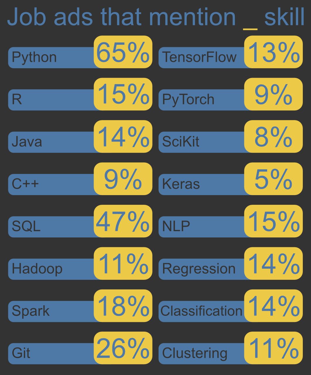
These numbers give a sense of the relative importance of the indicated skills, but it is important to keep in mind that we made a lot of simplifying assumptions in our analysis (covered below). So, these numbers should be taken with a grain of salt.

6. Limitations

Here we performed a quick analysis of job skills in Data Science postings. What we looked at was a back-of-the-envelope approximation. There are a number of ways we could be more thorough.

1. Diversify and expand our data. We only pulled job data from Indeed over a brief period of time. It would be helpful to draw data from other job boards over an extended period of time.
2. Screen our data more carefully. We identified important job skills by determining the percentage of job descriptions that contained certain keywords. One weakness of this approach was that we used an existing list of keywords. It may have been helpful to first search postings for common words or phrases to identify what keywords we should have used. Another weakness was that we did not test whether our keywords were associated with negative language. For instance, if the posting said "python skills are not required", we would have labeled that job ad as requiring python because the keyword occurred.
3. The text of the posting may not tell the whole story. For one, synonyms interfere with analysis. For two, some characteristics may be under represented in the text of job descriptions but still be important. For instance, the word curiosity only occurs in 134 posts, but I think most businesses want their data scientists to be curious!
4. Data science is a broad field. We cast the net broadly here on purpose, but it is important to keep in mind that the analyzed jobs span a wide range of titles (e.g., "Data scientist" to "Mathematical Technician"), seniority, etc.

7. Some other interesting tidbits

There are a lot of interesting insights to pull from these job postings. Here, we'll have a quick look at a few.

Commonly occurring words or phrases

With a few extra lines of code, and some natural language processing, we can have a look at the most commonly occurring words or phrases (n-grams).

First, we import the necessary libraries and store our job-scrape data in a DataFrame.

import pandas as pd
from nltk import everygrams, FreqDist
from nltk.corpus import stopwords
from nltk.stem import WordNetLemmatizer
lem = WordNetLemmatizer()

df = pd.read_feather('jobs.ftr')

Next, we want to process the text in our description. In this code, we add spaces before capital letters (this is because some of these spaces were removed when we scrapped the data), remove most punctuation, split the description string into a list of single-word strings, combine all lists of strings into a single list, and covert letters to lower case.

unigrams  = (
df['Description'].str.replace(r"(?<![A-Z])(?<!^)([A-Z])",r" \1",regex = True)
.str.translate(str.maketrans('', '', ',.!&:()'))
.str.split(expand=True)
.stack()
.str.lower()
).reset_index(drop=True)

Then, we remove stop words (e.g., and, was, any) and lemmatize.

unigrams = unigrams[~unigrams.isin(stop_words)]
unigrams_lem = [lem.lemmatize(w) for w in unigrams]

Finally, we can search for the n-grams. In this case, we look for the most common words or phrases that have between 1 and 3 words.

ngram = list( everygrams(unigrams, 1, 3) )
fdist = FreqDist(ngram)
out = pd.DataFrame(fdist.most_common(3000), columns=['Phrase', 'Frequency'])

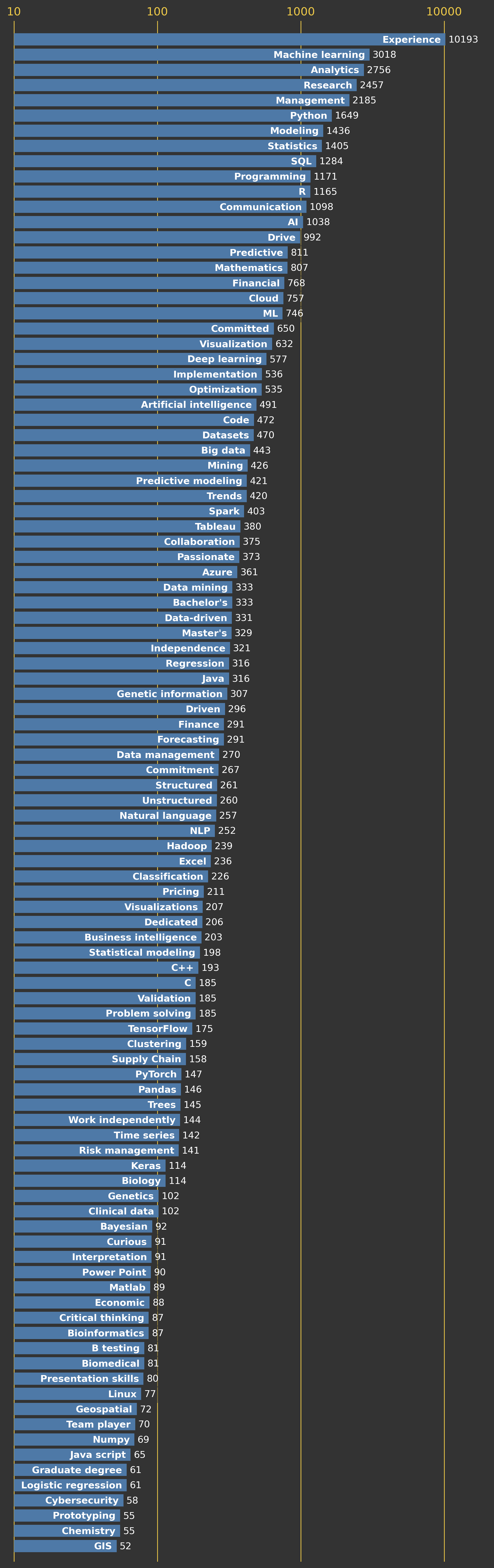
We can search our results above and pull out words/phrases of interest. Below, I show the frequency of job-skill related words in our 1920. These data were also used to create the word cloud at the top of this post.

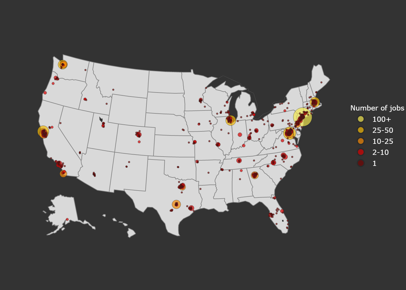
Where are the jobs?

We can also look at where the jobs are located. To create the bubble plot of job locations below, I used plotly. The process was somewhat complicated by the fact that the job locations did not have latitudes and longitudes. So, I downloaded coordinates for US cities here. We also have to remove some pesky punctuation. After doing that, we try to find a zip code associated with the job, if there is no zip code, we base our search off the city and state. Below is the code.

d = df.Location.str.replace('•', ' ').str.replace('+', ' ')
lat = []
long = []
misses = 0
for ind,loc in d.iteritems():
    zips = re.findall('\D(\d{5})\D', ' '+loc+' ')
    try:
        l = c[ c.Zip == int(zips[0]) ].iloc[0]
        lat.append( l.Lat )
        long.append( l.Long )
    except:
        city = loc.split(',')
        try:
            state = city[1].split()
            state = state[0]
            city = city[0].split('-')[0]
            if city == 'Manhattan':
                city = 'New York'
            elif city == 'St. Louis':
                city = 'Saint Louis'
            elif 'San Francisco' in city or 'Bay Area' in city:
                city = 'San Francisco'
            l = c[ (c.State_Code == state) & (c.City == city) ].iloc[0]
            lat.append( l.Lat )
            long.append( l.Long )
        except:
            if 'Remote' not in loc:
                misses += 1
out = pd.DataFrame()
out['Lat'] = lat
out['Long'] = long
out_freq = out.value_counts().reset_index(drop=True)

Now, we have our results! In the map below, the marker size and color indicate the number of jobs in a given location.

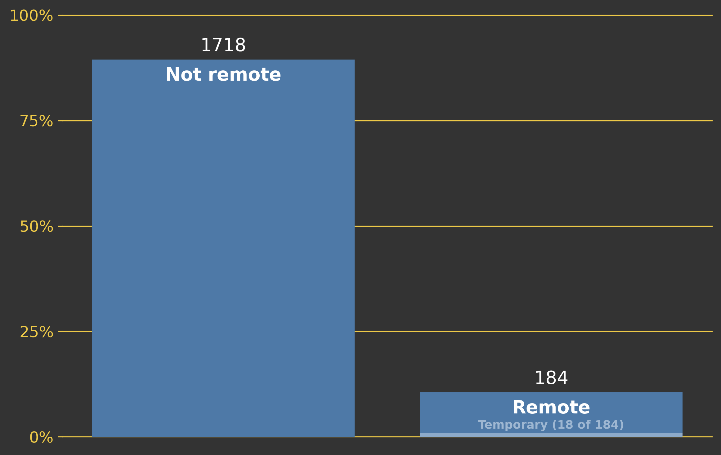
We can also consider how many of the jobs are remote. I did this by simply searching for the term "remote" in the location. I should note that some of the jobs are described as being remote in the description. So, our analysis will miss these jobs.